Analysing E-coli division

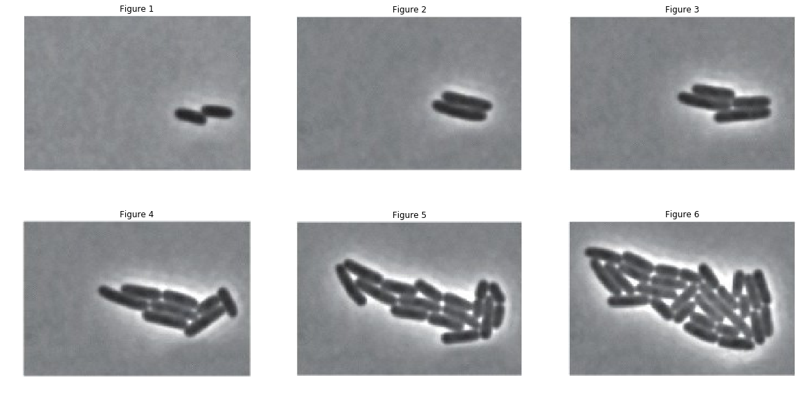
Here, we use image processing to analyse the growth pattern of bacteria from essential first principles. We use 6 images of a bacterial culture, taken at half hour intervals. In the following exercise, we will crudely estimate the number of bacteria in each image using the area occupied by the bacteria. This is a crude method because each bacterial cell isn’t the same size. However, if we assume that the variation in cell sizes isn’t very large, we can conclude that the area occupied is a very good indicator of the number of cells.

To read and analyze images, we need to import a module that has routines which are capable of performing the operations we require. One such library is scikit-image. We will also require numpy for various calculations and matplotlib for visualization

%pylab inline
import skimage
import skimage.io as io

Reading in the images

Let’s read the images using python now. The I/O submodule of scikit-image handles file I/O for most image formats. Our images are in the JPEG format. The imread() method reads image files and stores the value for each pixel in a numpy array. We can use Maplotlib’s imshow() method to display these images.

fig = plt.figure(figsize=(20,10))

images = []

for i in range(1,7):
    image = io.imread('./gc'+str(i)+'.jpg')
    images.append(image)
    # The figure is divided into a 2x3 grid
    subplot(230+i) 
    axis('off')
    title("Figure " + str(i))
    plt.imshow(images[-1]) ## Displaying images

To measure how fast E. Coli divides, we need to measure how much E. Coli there is in each picture. To do this, we need to differentiate between the bacterial cells and the background. This is a common task in image processing called segmentation. This is natural for your eyes but slightly more involved in computer science.

Even thought these images have RGB channels, it’s obvious that they’re in grayscale. We should convert them to true grayscale using the rgb2gray() method in the color submodule of scikit-image.

With these images now in grayscale, each pixel is just a number between 0 and 225 signifying the brightness. An intuitive way to differentiate between the cells and the background is by filtering brightness. The cells seem to correspond to the darker pixels in the images. Let’s plot histograms of these images and examine this further.

fig = plt.figure(figsize=(20,10))
plt.suptitle('Distribution of pixel brightness')

grayimages = []

for index, image in enumerate(images):
    grayimage = skimage.color.rgb2gray(image) 
    grayimages.append(grayimage)
    subplot(231+index)
    plt.hist(grayimage)
    plt.xlabel('Brightness (0=black, 1 = white)')
    plt.ylabel('Count')
    plt.title('Figure ' + str(index+1))

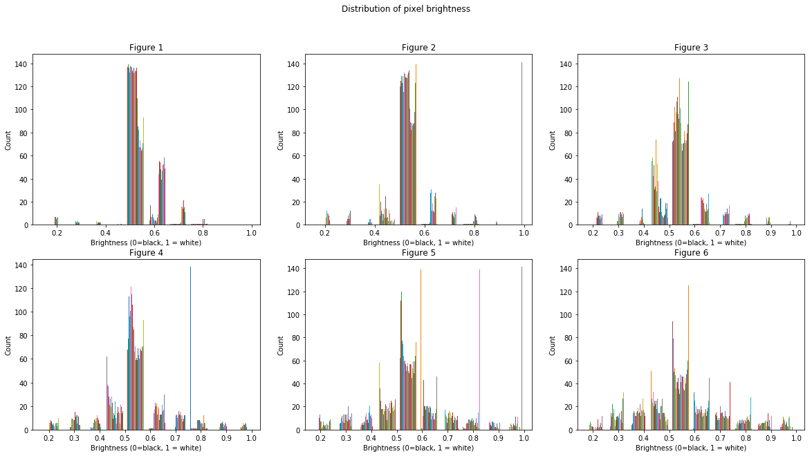
Let’s draw some conclusions from these histograms:

1. A majority of the pixels in each image has a brightness around half the maximum value.
2. The number of pixels falls off on both sides of the central lobe.

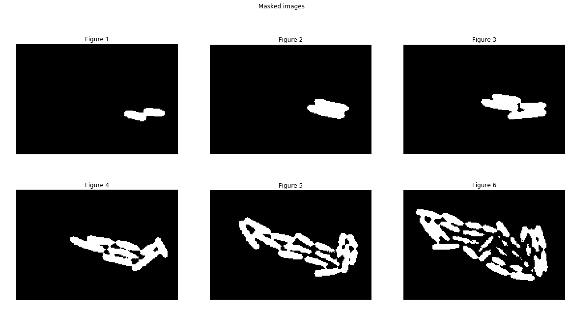
A logical thing to do would be to cut off any pixels with brightness including or above the central lobe. This should ideally only give us the pixels containing the cells. This technique is called thresholding. Let’s set 0.4 as our threshold brightness. (We’ve alrady tried different values for the threshold and 0.4 is optimal)

fig = plt.figure(figsize=(20,10))
plt.suptitle('Masked images')

for index, grayimage in enumerate(grayimages):
    mask = (grayimage < 0.4) 
    subplot(231 + index)
    axis('off')
    plt.imshow(mask, cmap ='gray')
    plt.title('Figure ' + str(index + 1))

Area calculations

Voila! The white areas roughly correspond to the E. Coli cells. Now we just need to count the number of such cells. This is easy becuase these masked arrays are just boolean values. A white pixel is a 1 and a black pixel is a 0. So counting white pixels is the same as summing up all the pixels in an image. Let’s measure how the percentage area occupied by the cells changes with time.

## defining time matrix
t= np.linspace(0,150,6)
area_perc = []

for index, grayimage in enumerate(grayimages):
    mask = (grayimage < 0.4) 
    occupied_area = np.sum(mask)
    total_area = grayimage.shape[0]*grayimage.shape[1]
    area_perc.append(occupied_area/total_area)
    
plot(t,area_perc,'bo')
title("Percentage Area occupied by E. Coli")
xlabel("Time in min.")
ylabel("Percentage area");

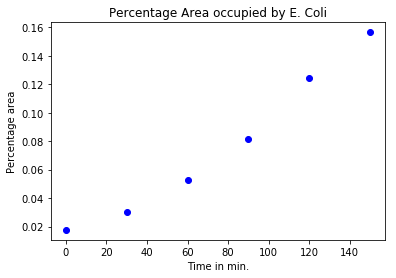
We can see that the percentage area increases roughly exponentially. Now to determine the doubling time, we need to fit an exponential distribution to these numbers and find the rate constant. An easy way to do this is to take the natural logarithm of our exponential data and then fit a straight line to it.

fittable = np.log(area_perc)
params = np.polyfit(t,fittable,1)

The variable params contains the parameters for the fitted curve. We now use these parameters to fit an exponential to our data. Here’s a visual representation of the fitting.

x = linspace(0,150,500)
plot(x,np.exp(params[0]*x+ params[1]),'k-')
plot(t,area_perc,'bo')
title("Percentage Area occupied by E. Coli")
xlabel("Time in min.")
ylabel("Percentage area")
legend(["Fitted curve","Experimental data"]);

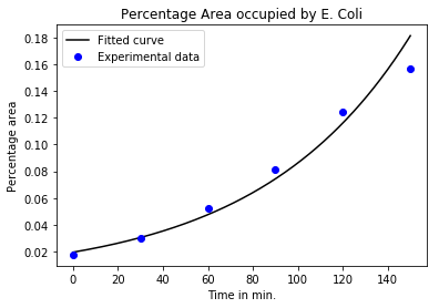
From the analysis of exponential curves, we know that the doubling time for the curve $Ae^{kt}$ is [ t_{double} = \frac{ln(2)}{k} ] so in this case:

Doubling time is 46.7 minutes

So this batch of E. coli doubles roughly every 47 minutes. The reason we can conclude on the doubling time from analysing area is because we can consider doubling of area to signify doubling of bacterial cells.